Data preparation, where to get a list of all NYSE and NASDAQ stocks (drl4t-03)

The key to machine learning is data. In order to train a machine learning model for predicting trading trends, we need to obtain as much historical trading data as possible.

The official NASDAQ website provides a reliable and cost-free resource in its stock screener page, which enables you to obtain a comprehensive list of stocks traded across all three major stock exchanges, NASDAQ, NYSE, and AMEX. You can access the page using this URL:

https://www.nasdaq.com/market-activity/stocks/screener

To illustrate, I downloaded a list of 23 large companies whose stocks are traded on NYSE and saved it as a file named nyse.csv. The data in this file includes the stock symbols, which we can use to obtain historical trading data of all these stocks using yfinance to train the machine learning models.

Read csv File

It’s very simple to read csv file using Pandas:

import pandas as pd

df = pd.read_csv('nyse.csv')

Download Trading Data

The “Symbol” column of the csv file contains the stock symbols we need. Using a loop, the historical trading data of each stock can be obtained by using yfinance as described in Acquiring data, the first step towards using machine learning for stock trading (drl4t-01). The script below gets the daily trading data of the last five years for each stock, excluding dividends and splits. The data has been stored in a directory.

import yfinance as yf

data = {}
for symbol in df['Symbol']:
    try:
        ticker = yf.Ticker(symbol)
        hist = ticker.history(interval='1d', period='5y', actions=False)
        if len(hist) > 0:
            data[symbol] = hist
    except:
        print(f'Failed to download data for {symbol}')

Not all stocks are active, and those that have not downloaded any trading data have been filtered out. The key of the directory includes a list of symbols of all active stocks.

data.keys()

Calculate Technical indicators

The technical indicators for each stock can be calculated as described in Technical indicators, tools for predicting trading market trends (drl4t-02).

for symbol, hist in data.items():
    hist['SMA10'] = hist['Close'].rolling(window=10).mean()
    hist['SMA20'] = hist['Close'].rolling(window=20).mean()
    
    ema_short = hist['Close'].ewm(span=12, adjust=False).mean()
    ema_long = hist['Close'].ewm(span=26, adjust=False).mean()
    hist['MACD_DIF'] = ema_short - ema_long
    hist['MACD_SIGNAL'] = hist['MACD_DIF'].ewm(span=9, adjust=False).mean()
    hist['MACD'] = hist['MACD_DIF'] - hist['MACD_SIGNAL']
    
    sma = hist['Close'].rolling(window=20).mean()
    std = hist['Close'].rolling(window=20).std()
    hist['UB'] = sma + 2 * std
    hist['LB'] = sma - 2 * std
    
    mfm = ((hist['Close'] - hist['Low']) - (hist['High'] - hist['Close'])) / (hist['High'] - hist['Low'])
    mfv = mfm * hist['Volume']
    hist['CMF'] = mfv.rolling(21).sum() / hist['Volume'].rolling(21).sum()

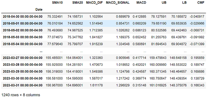
Let’s take a look at the data of the first stock with the following script. First, let’s get the symbol of the first stock:

symbol = list(data.keys())[0]

Then let’s check the technical indicators of this stock:

data[symbol][['SMA10', 'SMA20', 'MACD_DIF', 'MACD_SIGNAL', 'MACD', 'UB', 'LB', 'CMF']]

From this piece of data, two obvious problems can be seen, the NaN value and the data of different scales.

Data Normalization

As can be seen from the data above, both Simple Moving Averages (SMA) and Bollinger Bands (BB) values are correlated with the stock’s prices. They will vary greatly from stock to stock and cannot be used directly for machine learning.

Data normalization is to adjust values at different scales to a notionally common scale, often [0,1]. In this way, valid comparisons can be made between different ranges of data.

For Simple Moving Average (SMA), the simplest approach is to use the ratio of Close to SMA.

for symbol, hist in data.items():
    hist['SMARatio10'] = hist['Close'] / hist['SMA10']
    hist['SMARatio20'] = hist['Close'] / hist['SMA20']

For Bollinger Bands (BB), we can use the position of Close relative to the upper and lower bands. This is also known as the Bollinger Bands Position (BBP).

for symbol, hist in data.items():
    hist['BBP'] = (hist['Close'] - hist['LB']) / (hist['UB'] - hist['LB'])

Remove Data with NaN Values

The calculation of technical indicators often involves the average of rolling data. This will cause the results of the first few periods to be NaN because there is not enough data.

These trading data containing NaN values need to be removed. This is very simple with Python:

for symbol, hist in data.items():
    data[symbol] = hist.dropna()

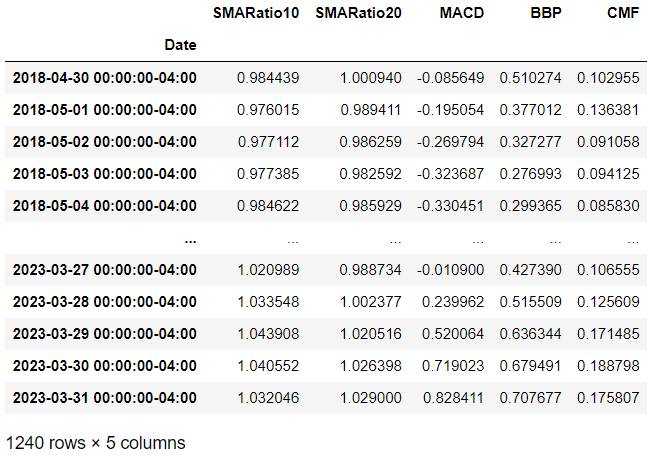
Data Ready

Now, let’s take a look at the first stock’s trading data after the whole data preprocessing completed:

data[symbol][['SMARatio10', 'SMARatio20', 'MACD', 'BBP', 'CMF']]

Split Data for Model Validation

The data is ready. But not all the it can be used directly to train the trading model. This is because a part of the data has to be reserved for model validation purposes.

There are two categories of techniques used for validating models: hold-out validation and cross-validation. When it comes to trading models, a form of hold-out validation known as back-testing is typically utilized. Essentially, back-testing involves partitioning historical trading data into two portions based on a chosen date. The older data is used for model training, whereas the more recent data is used for model validation.

The following script creates two new directories, train_data and test_data. Then, each stock’s trading data is split into two parts: earlier than split_date and equal or later than split_date. Here split_date is a trading day we can specify.

import datetime as dt

train_data = {}
test_data = {}

split_date = dt.date.today() - pd.DateOffset(days=100)

for symbol, hist in data.items():
    train_data[symbol] = hist[:split_date - pd.Timedelta(days=1)]
    test_data[symbol] = hist[split_date:]

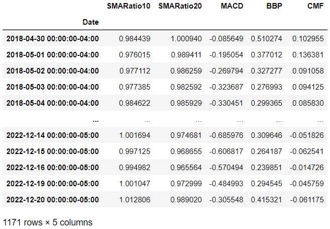
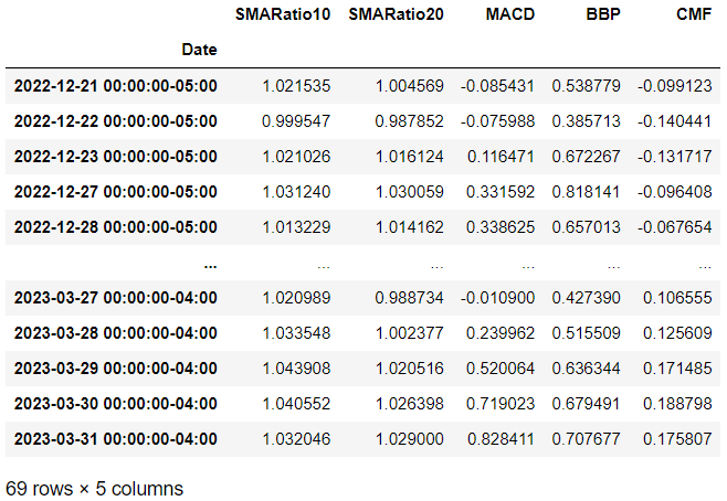
Now let’s check the training data and testing data of the fist stock. Pay attention to each of their date ranges and row counts.

train_data[symbol][['SMARatio10', 'SMARatio20', 'MACD', 'BBP', 'CMF']]

test_data[symbol][['SMARatio10', 'SMARatio20', 'MACD', 'BBP', 'CMF']]